Analyzing an algorithm is to determine how much resources the algorithm needs. The resources might be either memory usage, computational time, or network resources. This post will only focus on the computation time resource.
Computational time
Computational time is the time needed for an algorithm to do its processing.
Because an algorithm is eventually transformed into the basic operations provided by the hosting machine, its computational time is a function of the computation time of those basic operations. Because of this relationship, the RAM model is usually used as the hosting machine to simplify the computational time analysis. In this model, each basic operation (e.g., arithmetic, data movement, control, subroutine call and return) takes a constant amount of time [1, Sec. 2.2].
The computational time of an algorithm is also affected by the characteristics of the algorithm input, among which the most relevant one is the size of the input. For example, the computational time of an insertion sort algorithm increases as the number of items increases, and given a number of items to be sorted, the algorithm takes the longest time when the items are in the reverse order of the desired order.
Order of growth (or Rate of growth)
The order of growth of an algorithm tells us how quickly the computational time of the algorithm increases with the size of its input.
Order of growth is usually represented by asymptotic notations containing only the leading term (without its coefficient) of the computational time formula.
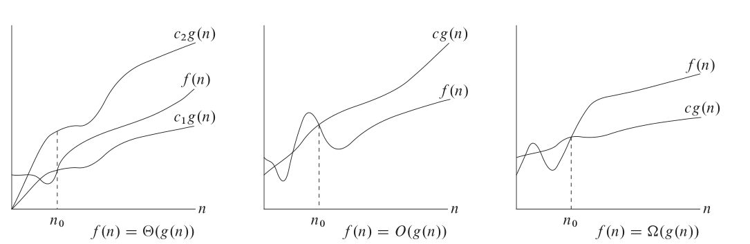 (Image source: [1, Fig. 3.1])
There are several advantages of using asymptotic notations over the exact computational time. First, it is easier to establish the asymptotic computational time. Second, it makes it simple to compare the computational time of different algorithms. And third, asymptotic notations fit well into the common situations where the main interest is to know how an algorithm performs as the input size increases.
However, asymptotic notations sometimes do not provide accurate judgement on the computational time when the input size is small. This is because these notations contain only the leading term of the computational time, which does not dominate the other terms when the input size is small. For example, given that the computational time of functions f and g are C(f) = n + 100 and C(g) = n^2 + 1, then even though C(f) = O(n) and C(g) = O(n^2), C(f) > C(g) for n < 10.
Types of analyses
Best-case analysis
This analysis focuses on the shortest time an algorithm might take for a given input size.
Worst-case analysis
This analysis focuses on the longest time an algorithm might take for a given input size.
Average-case analysis
This analysis focuses on the average time an algorithm might take for a given input size. It typically uses probability to analyze the average time.
Amortized analysis
This analysis focuses on the amortized cost of an algorithm. The amortized cost of a sequence of operations, which might contain different types of operations, is defined as the average cost of that sequence of operations. Thus, if a sequence of n operations takes T time, its amortized cost is T/n time.
This analysis usually gives a tighter bound on the computational time of a given sequence of operations than the worst-case analysis, which is mainly because amortized analysis takes into account the relationship between the operations in the sequence. For example, let consider a sequence of n stack operations, including push, pop, and popAll, on an initially empty stack. In worst-case analysis, this sequence takes O(n^2) time as it might have n popAll operations each of which might pop O(n) items in the worst case. However, in amortized analysis, this sequence only takes O(n) time, because the number of items popped out must be the same as that pushed into the stack and thus both of them are bounded by n.
It is important to keep in mind that amortized cost is about the average cost of an entire sequence of operations, not about any single operation. In the example above, it is valid to say that the amortized cost of n stack operations is O(1), but it is invalid to say that the amortized cost of any stack operation, either push, pop, or popAll, is O(1).
In its essence, amortized analysis exploits the relationship between the operations in the given sequence in such a way that the low costs of cheap operations compensate for the high costs of expensive operations. As a result, this analysis is able to give a tight average cost of the entire sequence.
Further reading
[1] Chapter 17, Introduction to algorithms